A temperature instability in our FEM model

The geometry

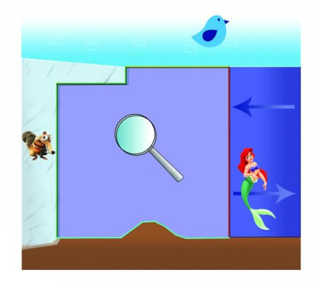
The simulation domain is 30×1 km, depicting a fjord. The right boundary faces the open ocean, the horizontal top boundary faces the atmosphere, the bottom is the bedrock, the tiny bottom-left vertical boundary stands for a small patch of land, and finally the slanted top-left boundary represents the ice-ocean interface.

On the side is a picture from a square version of the domain and a non-slanted ice shelf that might help render the idea.

Equations

On this domain, we solve the Navier-Stokes equations where the buoyancy force is given as a linear combination of temperature T and salinity S:

$\frac{\partial \textbf{u}}{\partial t} + \textbf{u} \cdot \nabla \textbf{u} = - \frac{\nabla p}{\rho_0} + \nu \nabla^2 \textbf{u} + \underbrace{(1 - \beta \Delta T + \gamma \Delta S) \textbf{g}}_{Buoyancy \ term}, \ \ \ \nu = \frac{\mu}{\rho_0}$

from which we obtain velocity and pressure profiles of the ocean. Temperature and salinity are solved for separately:

$\frac{\partial T}{\partial t} = \alpha \ \nabla^2 T - \nabla \cdot (\textbf{u}T)$

$\frac{\partial S}{\partial t} = \alpha \ \nabla^2 S - \nabla \cdot (\textbf{u}S)$

Both $\alpha$ and $\nu$ are constant vectors, accounting for the different viscosity/diffusion in horizontal and vertical directions.

For all the equations above, the weak form is derived so that a FEM formulation can be obtained. We also apply stabilization techniques to both the Navier-Stokes and the T/S equations (GLS for the former, SUPG for the latter). I leave these final equations out of the explanations voluntarily to save you time at this stage, and focus only on the setup we have.

Our implementation is in Python and is based on the FEniCS framework, which provides a toolkit to solve the FEM forms.

We use 2nd degree elements for velocity, while 1st degree elements for pressure, temperature and salinity.

Initial conditions

Temperature and salinity are initialized as stratified with values ranging from -1.6 to 0.4 °C for T, and from 34 to 35 PSU for S. This mimics the actual physical scenario.

Velocity and pressure are initialized to zero everywhere.

Boundary conditions

Boundary conditions are set to reflect the physical scenario.

Velocity is no-slip on all boundaries, except on the atmosphere interface, where motion is allowed x-wise. (The open ocean boundary is also no-slip, although it should be do-nothing, future project).
Pressure is set to zero on a point on the atmosphere interface.
Temperature/Salinity has insulated conditions on most boundaries (i.e. no flow) except on the ice-ocean interface, where a heat/salinity flux term plays the role of a Neumann condition mimicking influx of cold/fresh water coming from the melting ice. The open ocean boundary has instead a Dirichlet condition that matches the initial conditions.

The issue we are seeing

We have so far run the above scenario for 10 days of real-world time. The actual steady state is more around 50-60 days, but we haven’t yet run that long.

What follows is the evolution of the x-velocity and a close-up to a region of interest:

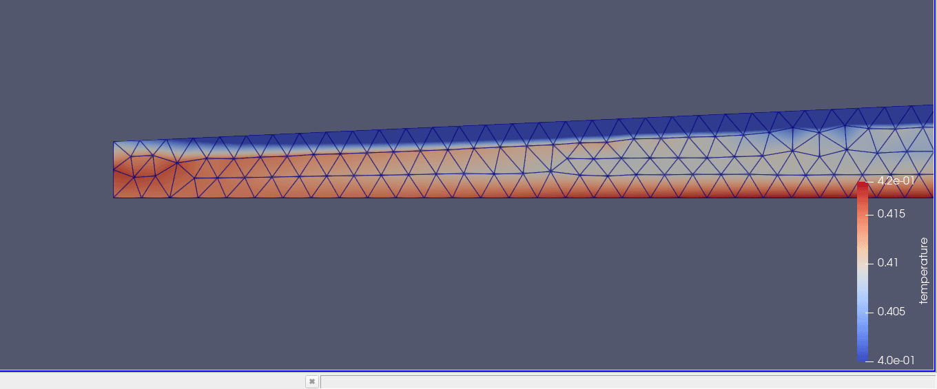
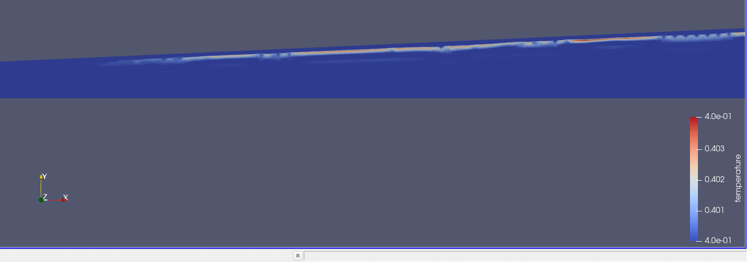
The issue that we are seeing is an overshot of temperature and salinity values in the proximity of the ice shelf, where the influx of colder and fresher water is. The next animations show the temperature evolution for values in the range of the overshot $T \in [0.4, max]$ ; in other words, it only shows values above the expected maximum. Salinity exhibits a very similar behavior, except with different values.

My own interpretation is that the large gradient generated by the discontinuous jump between the boundary condition ( $T<0.4$ ) and the initial value ( $T=0.4$ for the most part). This causes in turn the solution to overshoot just after the cool/fresh boundary layer.

On the largest part of the domain, this slight inaccuracy soon diffuses away and doesn’t generate much problems, but on the left part of the domain, where both the vertical left boundary and the bottom boundary have no-flux boundary conditions, the extra heat diffuses in the x-direction and results, in the long term, in a sliver of warm+fresh water all alongside the bedrock, which in turn generates spurious velocities down there. The combination of fresh+warm water is heavier than the surrounding area, so it doesn’t rise and stays at the bottom.

After 10 days, T reaches up to 0.42 degrees in that area, which is a 2% error. Given that there is no sign that this overshot would die out with further simulation time, it is reasonable to believe that, after 50 days, the error would be around 10% – grossly inaccurate.

What feels even weirder is that, in the bottom-left region, this overshot does not die out in time as it does on the rest of the ice shelf. It almost looks like there is a heat source from that left boundary.

Further comments & prospective solutions

We have confirmed that the issue really comes from the boundary conditions. Reasons to believe are that:
a) we observe a similar issue if we take away the flux terms and replace them with constant Dirichlet conditions, say with T = 0.39 and S = 34.9;
b) we have tried applying the flux conditions only on the upper half of the ice shelf, and we have seen no overshot in the bottom-left (although the shock-like behavior seen in the previous animations was still there, for the upper part).

For a simplified setup, where temperature and salinity were initialized as constant, instead of stratified as in this case, we tried making the initial conditions for T and S smoothly reach the boundary value, so that the boundary conditions would not create a discontinuous situation. This seemed to help a bit, but it’s hard to be sure also given the difference in setups – it’s something we should double check and retry.
We thought it could be due to an abrupt change in boundary conditions from no-flux on the left boundary, and some-flux on the ice shelf. However, making the flux terms smoothly go to zero towards the end of the boundary did not seem to help.
All throughout, we have used 2nd degree elements for velocity and 1st degree for pressure, temperature and salinity. Bumping everything up 1 degree (P3P2P2P2) did not seem to help, nor has the combination P3P2P1P1 performed better (this last setup seems to be able to solve some geometry-related instabilities, making the pressure and T/S elements compatible with each other).

At this point we turned towards Discontinuous Galerkin, in the hope that it would prevent that inaccuracy from building up in the first place. Given the insulated nature of the left and bottom boundaries, it seems like once a pocket of warmer water has been created, it will have a hard time being flushed, so a good approach seems to lie in avoiding this warmer water from showing up at all. Given the work involved in implementing DG, we gladly avoid pursuing this track if it doesn’t seem probable that it could be of help, of course. FEniCS, the framework we use, has some built-in stuff on DG, but our ignorance on the matter (and the poor documentation) makes it hard to evaluate how much there is and how much needs to be done, as well as the prospective benefits we could harvest from this change (also performance-wise).

Was this Helpful ?
yes no